· H2 Mathematics — Ten-Year Series, worked ← All 10 questions

2018 A-Level · Paper 2 · Question 9

2018 H2 Maths Paper 2, Question 9

Correlation and regression 12 marks regression lines
Download Paper 2 solutions (PDF)

Part (i)

2 marks
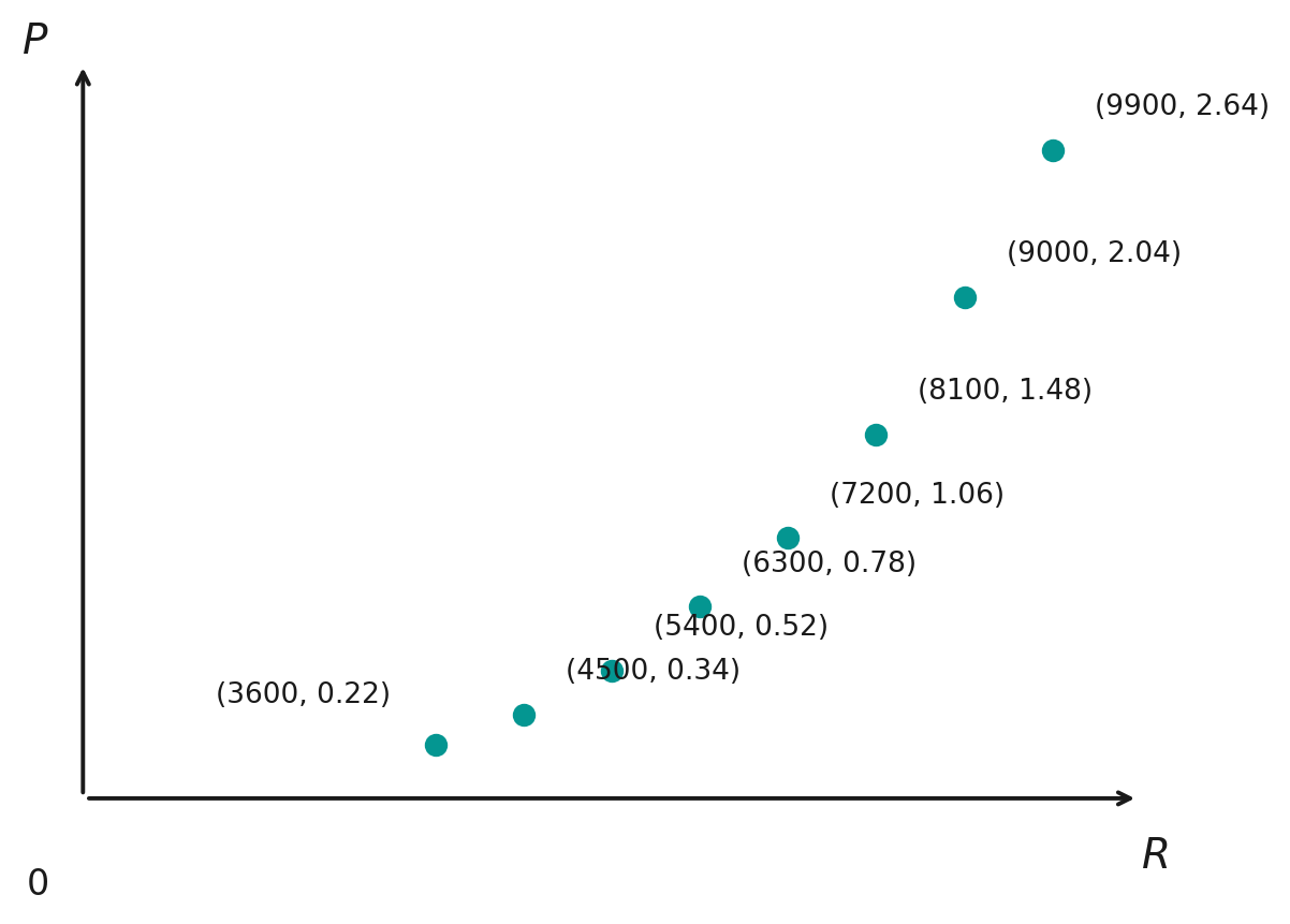
Sketch for question 9

The points do not lie close to a straight line — they curve upwards more and more steeply as RR increases, bending away from any single straight line through them. This suggests the relationship between PP and RR is not well modelled by P=aR+bP = aR + b; a curved (non-linear) model fits the pattern of the data better.

Part (ii)

6 marks

Approach

to compare the two proposed models, P=aR+bP = aR + b and P=aR2+bP = aR^{2} + b, we compute the product moment correlation coefficient (PMCC) for each — the first between PP and RR, the second between PP and R2R^{2} (since P=aR2+bP = aR^{2} + b is linear in R2R^{2}, not in RR) — and take the model whose rr is closer to 11.

By GC,

rP, R=0.969 (3 s.f., by GC)r_{P,\, R} = 0.969\ \text{(3 s.f., by GC)}
rP, R2=0.993 (3 s.f., by GC)r_{P,\, R^{2}} = 0.993\ \text{(3 s.f., by GC)}

Explanation: rP,R2=0.993r_{P,R^{2}} = 0.993 is closer to 11 than rP,R=0.969r_{P,R} = 0.969, so P=aR2+bP = aR^{2} + b gives a stronger linear relationship (between PP and R2R^{2}) than P=aR+bP = aR + b does (between PP and RR), and is therefore the better model.

By GC, the regression line of PP on R2R^{2} is

P=2.85×10⁻⁸R2−0.283 (3 s.f., by GC).P = 2.85 \times 10^{- 8}R^{2} - 0.283\ \text{(3 s.f., by GC).}

∴\therefore P=aR2+bP = aR^{2} + b is the better model, with a=2.85×10⁻⁸a = 2.85 \times 10^{- 8} and b=−0.283b = - 0.283, both correct to 3 s.f.

Part (iii)

2 marks

Using the equation from (ii), we solve for RR when P=0.9P = 0.9:

0.9=(2.845744…×10−8)R2−0.282608…0.9 = \left( 2.845744\ldots \times 10^{- 8} \right)R^{2} - 0.282608\ldots
⇒R2=0.9+0.282608…2.845744…×10−8\Rightarrow R^{2} = \frac{0.9 + 0.282608\ldots}{2.845744\ldots \times 10^{- 8}}
⇒R=6450 (3 s.f., by GC),\Rightarrow R = 6450\ \text{(3 s.f., by GC),}

taking the positive root since speed R>0R > 0.

Explanation: R=6450R = 6450 lies within the range of the given data (3600≤R≤99003600 \leq R \leq 9900), so this is an interpolation, and the estimate is reliable.

∴\therefore the estimated speed is R=6450 rpmR = 6450\ \text{rpm} (3 s.f.), and this estimate is reliable.

Part (iv)

2 marks

Using the equation from (ii), at R=3300R = 3300,

P=(2.845744…×10−8)(3300)2−0.282608…P = \left( 2.845744\ldots \times 10^{- 8} \right)(3300)^{2} - 0.282608\ldots
=0.0273 (3 s.f., by GC).= 0.0273\ \text{(3 s.f., by GC).}

Explanation: R=3300R = 3300 lies outside the range of the given data (3600≤R≤99003600 \leq R \leq 9900), so this is an extrapolation, and the estimate is unreliable — the equation is not known to hold below R=3600R = 3600.

∴\therefore the estimated power used is P=0.0273 wattsP = 0.0273\ \text{watts} (3 s.f.), but this estimate is unreliable since it extrapolates beyond the data.

Part (v)

Approach

the equation in (ii) uses RR in revolutions per minute. If rr denotes the speed in revolutions per second, then R=60rR = 60r (there are 6060 seconds in a minute), so we substitute R=60rR = 60r into the equation from (ii).

Let rr be the fan speed in revolutions per second, so R=60rR = 60r. Substituting into P=aR2+bP = aR^{2} + b from (ii),

P=a(60r)2+bP = a(60r)^{2} + b
=3600ar2+b= 3600ar^{2} + b

By GC, 3600a=3600×2.845744…×10−8=1.02×10−43600a = 3600 \times 2.845744\ldots \times 10^{- 8} = 1.02 \times 10^{- 4} (3 s.f.).

∴P=1.02×10⁻⁴r2−0.283\therefore P = 1.02 \times 10^{- 4}r^{2} - 0.283, correct to 3 s.f., where rr is the fan speed in revolutions per second.

This is how we mark, and how we teach.

Every Ten-Year Series question, worked in full, with the reasoning written out and the traps named.

Find out more