2017 H2 Maths Paper 2, Question 8

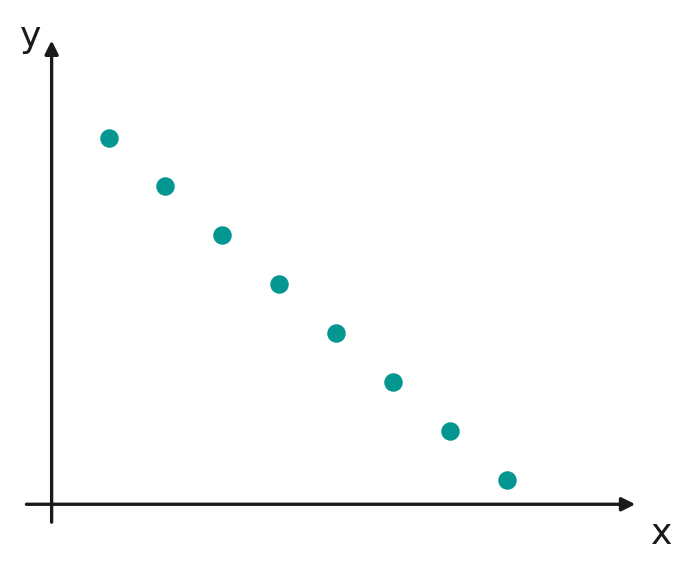
$r = - 1$: eight points lying exactly on a straight line of negative gradient.

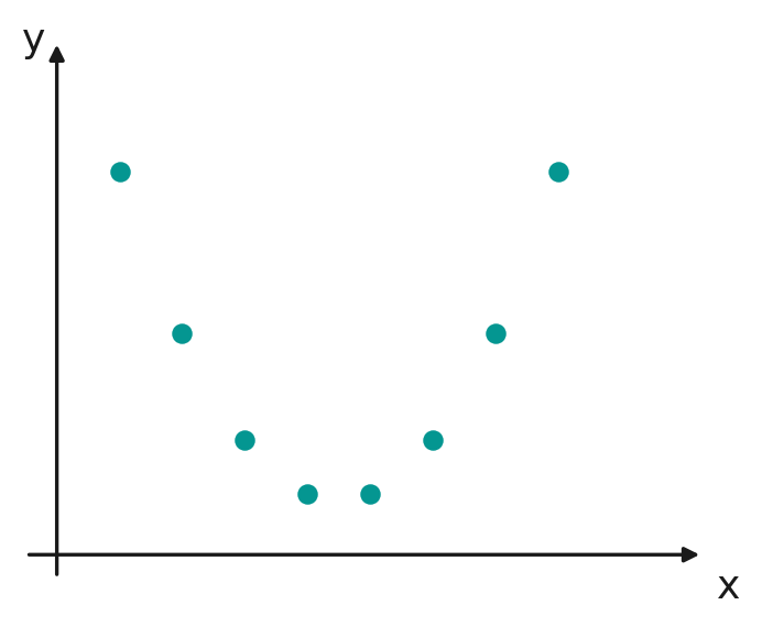
$r = 0$: eight points in a symmetric curved (non-linear) pattern, so that increases in $x$ are matched equally by increases and decreases in $y$, giving no net linear trend.

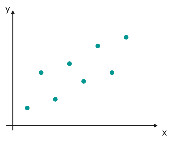
$0.5 < r < 0.9$: eight points showing a clear increasing trend, but with enough scatter about the underlying line that the fit is not near-perfect.

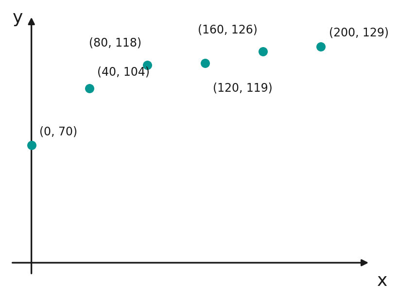
The scatter diagram shows $y$ increasing with $x$, but at a decreasing rate, levelling off as $x$ grows, with no sign of turning downward.

Note: $x = 0$ is one of the given data points. Models (B) $y = \frac{a}{x^{2}} + b$ and (C) $y = a\ln 2x + b$ are both undefined at $x = 0$, so neither can represent this data set at all. This leaves (A) $y = ax^{2} + b$ and (D) $y = a\sqrt{x} + b$ to compare.

By GC, the product moment correlation coefficients for the two remaining linearised models are

Since $\left| r_{\sqrt{x},\, y} \right|$ is much closer to $1$, and $y = ax^{2} + b$ would be increasing at an increasing rate (the opposite of the levelling-off pattern seen), model (D) $y = a\sqrt{x} + b$ provides the most accurate model.

Using model (D) with $x$ and $y$ as given, by GC (linear regression of $y$ on $\sqrt{x}$),

The product moment correlation coefficient for this model is

1. $x = 189$ lies within the range of the given data ($0 \leq x \leq 200$), so this is interpolation, not extrapolation, which is more reliable.
2. The product moment correlation coefficient $r = 0.981$ is close to $1$, showing a strong linear relationship between $\sqrt{x}$ and $y$, so the model fits the data well.